Cohort State-Transition Models (cSTM) for Cost Effectiveness Analysis
Introduction
A common tool used to project the long-term outcomes and costs of various policies, treatments, or other interventions in health economic analysis is the cohort state-transition model (cSTM). These models predict how a individuals in a hypothetical cohort transition between states over time, often health states when used in the context of health economics. cSTM are appropriate tools to use when one wants to model a dynamic process (i.e., evolving over time) in which there are transitions between discrete states. These models are often used to compare the costs and benefits of alternative interventions, and we will run through some examples of how to apply these models to these types of questions using R.
The “cohort” part of cSTM indicates that each theoretical cohort is considered homogeneous. There is another form of STM called individual STMs (iSTMs) that are more computationally demanding but can capture how time-varying variables impact the state-transition probabilities. We will focus solely on the simpler cSTMs for this post.
This document will pull largely from a tutorial in using cSTM for cost-effectiveness analysis (CEA) published by Alarid-Escudero et al. out of the Center for Research and Teaching in Economics (CIDE) in Mexico in 2022 (their code repo here). It will cover both time-independent and time-dependent forms of cSTM, and the later parts of the document will also cover later developments in state-transition models and their applications to economic analysis.
Additional discussion of best practices for STMs can be found in State-Transition Modeling: A Report of the ISPOR-SMDM Modeling Good Research Practices Task Force-3
Time-Independent cSTM: The Math
Basic concepts
STMs model how the number of individuals in each of a set of states evolves over time. These states are a finite set of mutually exclusive (i.e., no overlap) and completely exhaustive (i.e., no unmeasured/unobserved states) discrete values. In the case of discrete time steps, the states of a given time can be represented by a “state vector” \(m\) with individual entries for each of the number of states \(n_s\):
\[Equation 1: m_t=[m_{(t, 1)}, m_{(t, 2)}, ..., m_{(t, n_s)}]\]
\(n_s\) mutually exclusive states across \(n_t\) mutually exclusive discrete time cycles, usually of a fixed length (e.g., months or years), wherein individuals in each state are indistinguishable from one another. Probabilities \(p\) are assigned for transitioning between each combination of two states or staying within the same state over a given time cycle length. These probabilities are Markovian, which means that the probabilities are only dependent on the current state. This is why these models are also sometimes called “Markov models”.
As an example, if the probability of transitioning from the state “healthy” to the state “sick” is 0.02 over a one-year cycle, this means that the model assumes that everyone in the “healthy” state has the same 0.02 probability of transitioning into the “sick” state no matter at what time during that year or if they had been in the “sick” state prior to being in the “healthy” state or how long they’ve been in the “healthy” state, etc. The model simply assumes that the only factor impacting the probability is that current state.
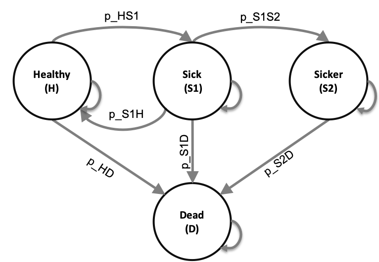
A popular STM framework common in CEA is the Decision Analysis in R for Technologies in Health (DARTH) 4-state (\(n_s=4\)) “Sick-Sicker Model”. Here patients transition between the states “Healthy (H)”, “Sick (S1)”, “Sicker (S2)”, and “Dead (D)”, with participants who reach the “Sicker” S2 state only either staying in that state or dying. Fig. 1 below shows how the states evolve, with probabilities of each transition being marked as \(p_{\zeta_1\zeta_2}\) where each \(\zeta_1\) is starting state and \(\zeta_2\) is the ending state. Not shown are the probabilities of remaining in the same state, for example the probability of remaining dead (\(p_{DD}\)), which is 100%.